Recognizing and Localizing Endangered Right Whales with Extremely Deep Neural Networks

In this post I’ll share my experience and explain my approach for the Kaggle Right Whale challenge. I managed to finish in 2nd place.

1. Background

Right whale is an endangered species with fewer than 500 left in the Atlantic Ocean. As part of an ongoing preservation effort, experienced marine scientists track them across the ocean to understand their behaviors, and monitor their health condition. The current process is quite time-consuming and laborious. It starts with photographing these whales during aerial surveys, selecting and importing the photos into a catalog, and finally the photos are compared against the known whales inside the catalog by trained researchers. Each right whale has unique callosity pattern on the whale head (see digram below). You can find more details at the competition page. The goal of the competition was to develop an automated process to identify the whales from aerial photos.

Image quality varies quite a bit because they were possibly taken in different years with different camera equipments. Note that some images were overexposed and some were underexposed. But in general, I found it very difficult to identify the whale myself with even using the highest quality images.

Here are 4 pairs of right whales, can you guess which ones are the same and which ones are not?

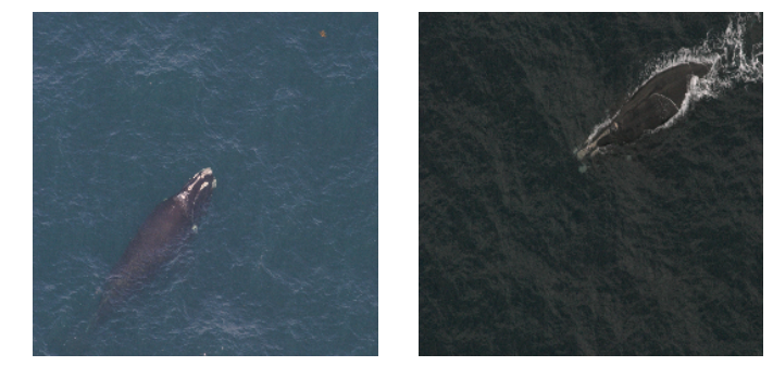
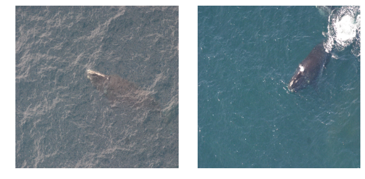
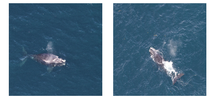
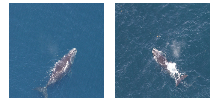
(Answers can be found from the URL of the images)

One thing that I didn’t notice from the images was how big these whales actually are. They can grow to 50 feet, weigh up to 170,000 lbs, and has a life span of typically 50 years. You can learn more fascinating facts about right whales from the NOAA website

2. Dataset

This dataset was special in 2 main ways from the perspective of machine learning.

2.1 Dataset distribution

It was non-straightforward to split the dataset into training and validation set. There were only 4237 images for 427 right whales. Most importantly the number of images per whales varies hugely, as can be seen from the below histogram. There were 24 whales that came with only 1 image in the dataset!

A reasonable local validation set was essential to evaluate how the model will perform on the testing set and estimation of public / private score on Kaggle.

The usual approach is to perform a stratified split so that the training and validation label distribution were similar. To handle the whales with single photo, we can either a) put those images just in the training set (overestimating); or b) just in the validation set (underestimate). Note that putting the whales with 1 image into validation set would result in the classifier not be able to predict those whales at all!

However due to a noob mistake, I ended up doing a random split. To makes things worse, different classifiers were trained with a different split. I noticed this issue about 3 weeks before the deadline, and I decided not to fix them because I thought it was too late.

Ironically none of model trained before that point ended up in the final submission. Lesson learned: it is never too late to makes thing right, just like in life.

2.2 Extremely fine-grained classification

Unlike many commonly cited classification tasks which is to classify images into different species (bird, tree leaves, dogs in ImageNet), this task is to classify images of the same species into different individuals. So the classifier must pick up the fine details of the callosity patterns regardless of image perspective and exposure etc.

Fortunately the academia has actually done immense work about recognition within a species – Homo sapiens. Realizing the similarity of recognition whale and human would become a source of many of my ideas.

3. Software and Hardware

Software

All code was written in Python. The neural networks were trained using Lasagne, Nolearn and cuDNN. scikit-image, pandas and scikit-learn were used for image processing, data processing and final ensembling respectively. I also made use of iPython / Jupyter notebook to sanity check my result and and ipywidgets to quickly browse through the images. Most of the charts in the blog post were made using matplotlib and seaborn.

Hardware

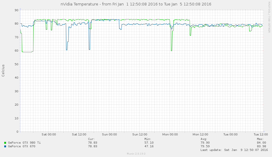
Most of the models were trained on GTX 980Ti and GTX 670 on a local Ubuntu machine. I made use of AWS EC2 near the very end of the competition, which will be explained further in Section 5.2

Who needs a heater when your machine is crunching numbers all the time!

4. Approaches

All my approaches were based on deep convolutional neural network (CNN), as I initially believed that human is no match to machine in extracting image feature. However it turned out that machines are not quite there yet. Understanding neural network performance bottleneck proved to be very important.

Below are 3 approaches I attempted in chronological order

4.1 Baseline Naive Approach

After deciding to participate in this competition, the first thing I did was to establish a baseline classifier with CNN.

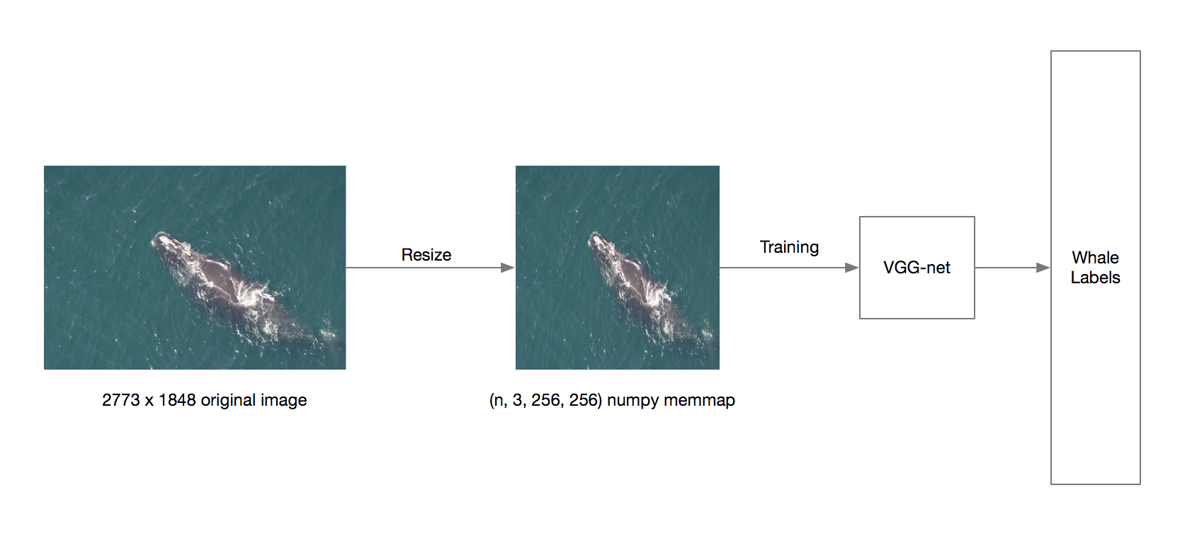
Virtually no image processing is performed, except to resize them to 256x256 and stored as numpy memmap. I did not even perform zero mean unit variance normalization. Also the aspect ratio is not preserved during the resize. The target of the model was the whale name encoded to 0 and 447 as integer. The network architecture was based on OxfordNet.

OxfordNet (or VGGNet) was the winner of the 2014 ImageNet challenge. It contained a series of stacks of small 3x3 convolutional filters immediately followed by max-pooling. The network usually ended with a few stacks of fully connected layers. See original paper for details.

The network was trained with heavy data augmentation, including rotation, translation, shearing and scaling. I also added “brightness” augmentation to account for underexposed and overexposed images. I found that color permutation did not help, which made sense because there was not much color variation in the images.

Very leaky rectified linear unit (VLeakyReLU) was used for all of the models.

This naive approach yielded a validation score of just ~5.8 (logloss, lower the better) which was barely better than a random guess. This surprised me because I expected the network to be able to focus on the whale given the non-cluttered background. My hypothesis for the low score was that the whale labels did not provide a strong enough training signal in this relatively small dataset.

To prove my hypothesis, I looked at the saliency map of the neural network that is analogous to eye tracking. This was done by sliding a black box around the image and keeping track of the probability changes.

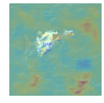
The saliency map suggested that the network was “looking at” the ocean waves instead of the whale head to identify the whale.

I further experimented with larger image sizes (e.g. 512x512) but found image size did not accuracy.

4.2 Bounding Box Localization

To help the classifier locating the whale head and hence improve the score, I added a localizer before the classifier.

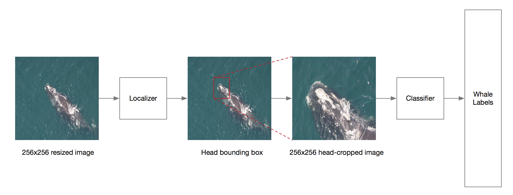
A localization CNN took the original photos as input and output a bounding box around the whale head, and the classifier was fed the cropped image.

This is made possible thanks to the annotations by Vinh Nguyen posted to the competition forum.

4.2.1 Localizer

I treated the localization problem as a regression problem, so that the objective of the localizer CNN is to minimize the mean squared error (MSE) between the predicted and actual bounding box. The bounding boxes were represented by x, y, width and height and were normalized into (0, 1) by dividing with the image size.

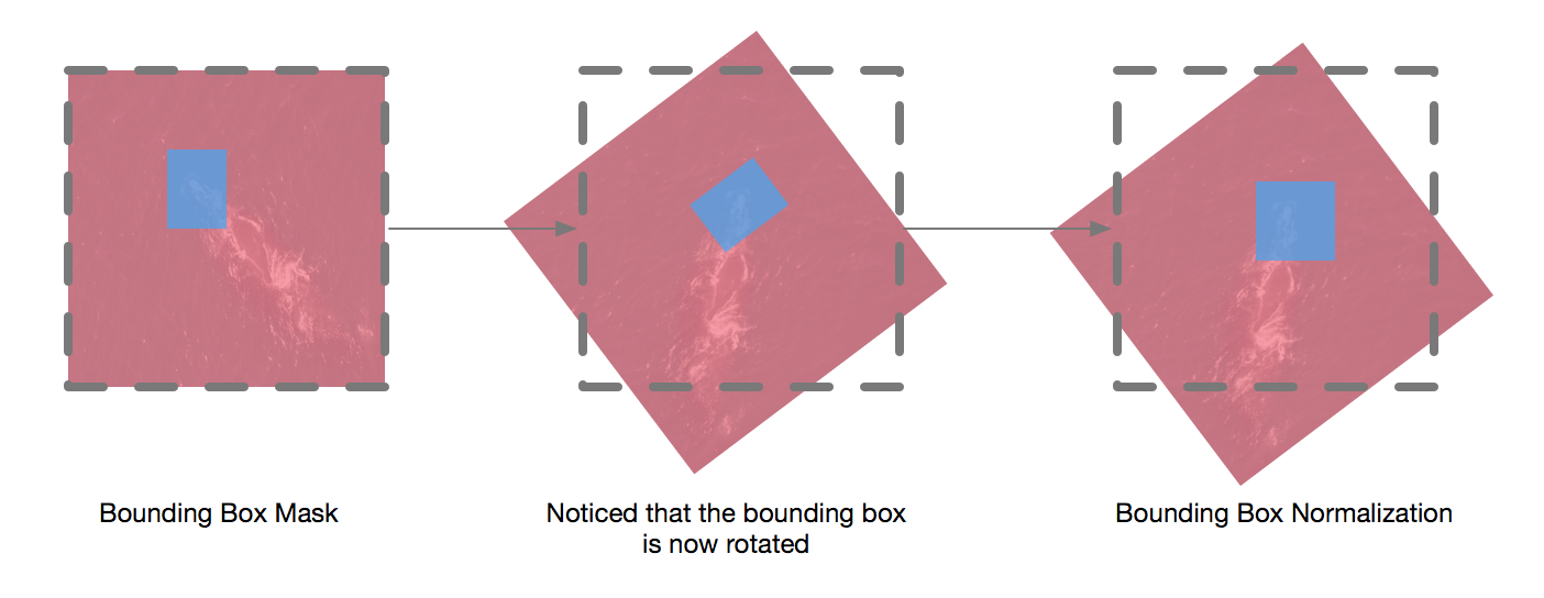
Similar to the baseline model, the network structure is based on OxfordNet. Data augmentation was applied to the images as well. To calculate the bounding box of the transformed image, I created a boolean mask denoting the bounding box, applied the transformation to this mask, and extracted the normalized bounding box from the mask. See diagram below for details.

The model took a long time to converge and slowed down significantly after 10% of the training time. I suspected that MSE with normalized coordinates was not ideal for regressing bounding boxes, but I could not find any alternative objective function from related literatures.

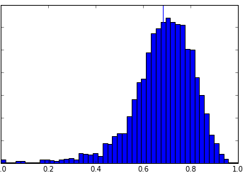
The more accurate metrics should measure the overlap between the actual and predicted bounding boxes. So I further evaluated the localizer with interaction over union (IOU) which is the ratio of the area of intersection the predicted and actual bounding boxes and area of their union. This metrics is based on Jacquard Index, ranges from 0 to 1 (higher the better).

The graph below shows the distribution of IOU between the actual and predicted bounding boxes.

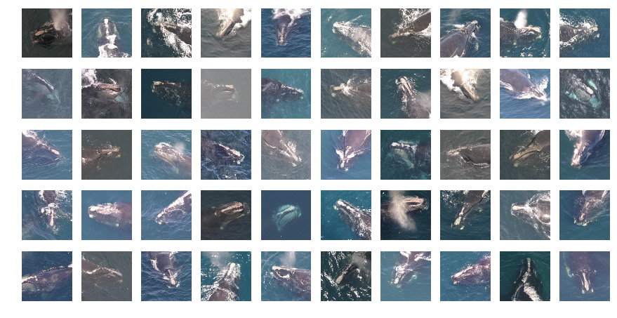
Below are samples of cropped images from the test set.

4.2.2 Classifier

The classifier for this approach was again a OxfordNet trained on cropped 256x256 images.

Ultimately this approach led to a validation score of about ~5, which was better than the naive approach but still not a significant improvement.

I experimented with the amount of padding around the predicted bounding box and found that it did not affect accuracy.

4.3 Whale Head Aligner

At this point, it was clear that the main performance bottleneck is that the classifier was not able to focus on the actual discriminating part of the whales (i.e. the callosity pattern). So in this approach, a new aligner replaced the localizer. Particularly, the aligner rotated the images so the whale’s bonnet would be always to the right the blowhead in the cropped image.

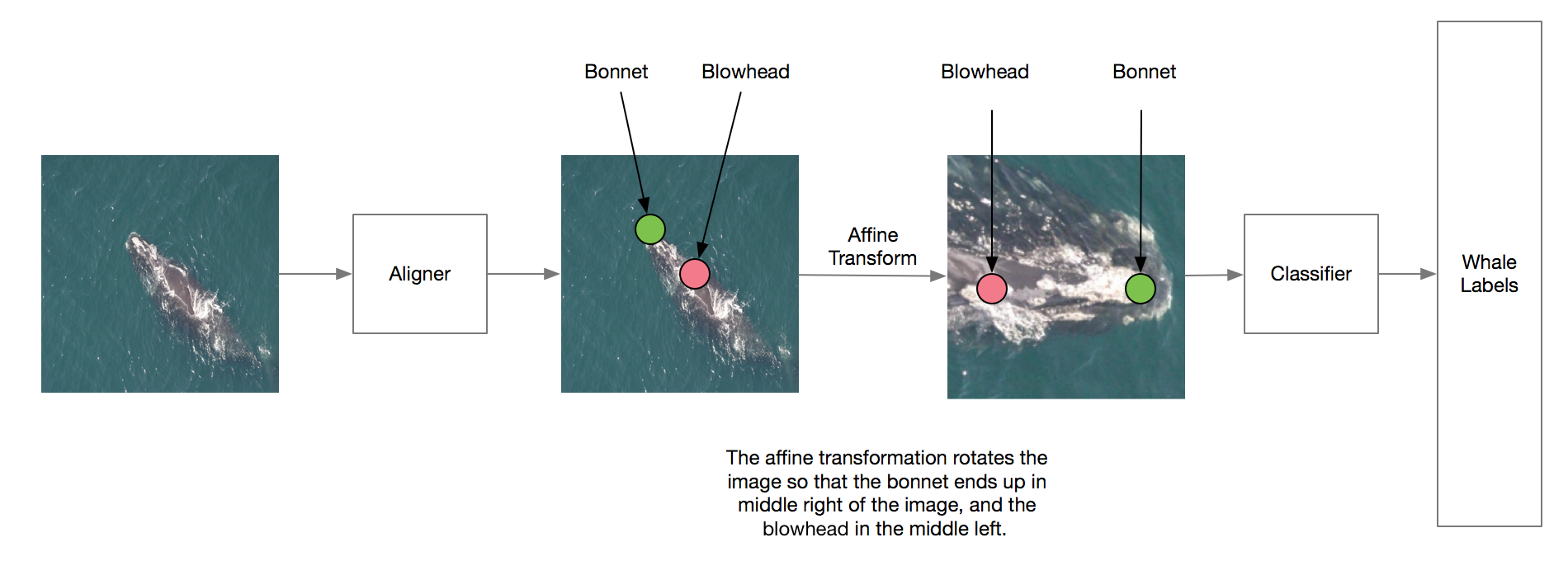
The head-cropped images were extracted by applying an affine transformation according to the predicted coordinates. This was made possible by the annotations from Anil Thomas.

While the architecture of this approach looked very similar to the previous one, the fact that the images were aligned had a huge implication for the classifier – the classifier no longer need to learn features which are invariant to extreme translation and rotation. However note that the aligned image were still not normalized by camera perspective, occlusion and exposure etc.

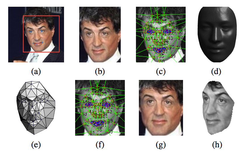
This approach somewhat reminded me of the Facebook’s DeepFace paper. DeepFace is a human face recognition system and it applied 3D frontalization to the face image before feeding it to the neural network. Obviously, it was not possible to perform similar alignment with just 2 points, but it was reasonable to assume that accuracy can be improved if there were more more annotation keypoints, as that would allow more non-linear transformation.

They also employed locally-connected convolutional layers, which different filters were learned at different pixel locations. However I did not ended up using the locally-connected convolutional layers in my models because simply the implementation in TheanoLinear doesn’t seem to be compatible the Theano version I am using.

4.3.1 Aligner

The aligner was again a OxfordNet-style network and its target was normalized x, y-coordinates of the bonnet and blowhead. Inspired by the recent papers related to face image recognition, I replaced the 2 stacks of fully connected layers with a global averaging layer, and used stride=2 convolution instead of max-pooling when reducing feature maps size. I also started to apply batch-normalization everywhere.

Heavy data augmentation was applied to prevent overfitting, which included rotation, translation, shearing and brightness adjustment. Note that the target coordinates needed to be adjusted accordingly too. This could be done by simply applying the affine transformation matrix to the coordinates.

Since the aligner was optimized with the MSE objective function similar to the previous approach, I observed similar slow convergence after about 10% of the training time.

I applied test-time augmentation and found that it helped the improving accuracy significantly. So, for each test image, I applied multiply affine transformations and then fed them into the aligner. I inverse applied the affine transformation to the predicted bonnet and blowhead coordinates and simply took the average of those coordinates.

4.3.2 Classifier

The main classifier I used in this approach was a similar 19-layers OxfordNet. I carried over the global averaging layer and stride=2 as max-pooling. The difference was that minimal augmentation was applied because both the training and testing images would be aligned. I empirically found that heavy augmentation prevented the network to converge, and lighter augmentation did not lead to overfitting. For similar reason, I did not apply test-time augmentation to the classifier.

Remember the noob mistake I mentioned at the start about making a local validation set? It turned out I randomly selected 20% of images for the aligner and 15% of data for the classifier. This meant some validation images for the classifier were part of the training set of the aligner and vice verse! This led to huge problems in validating classifier results, and I resorted to relying on the public leaderboard for validation! So lesson learned: Split your dataset right at the start and store your split separately!

5. More Experimentations

2 weeks before the deadline, I started to experiment with the state-of-the-art CNN structures. Some of them ended up being used in the final submission.

5.1 Deep Residual Network (ResNet)

The success of deep learning is usually attributed to the highly non-linear nature of neural network with stacks of layers. However the ResNet authors observed an counter-intuitive phenomenon – simply adding more layers to a neural network will increase training error. They hypothesized that it would be effective to encourage the network to learn the “residual error” instead of the original mapping.

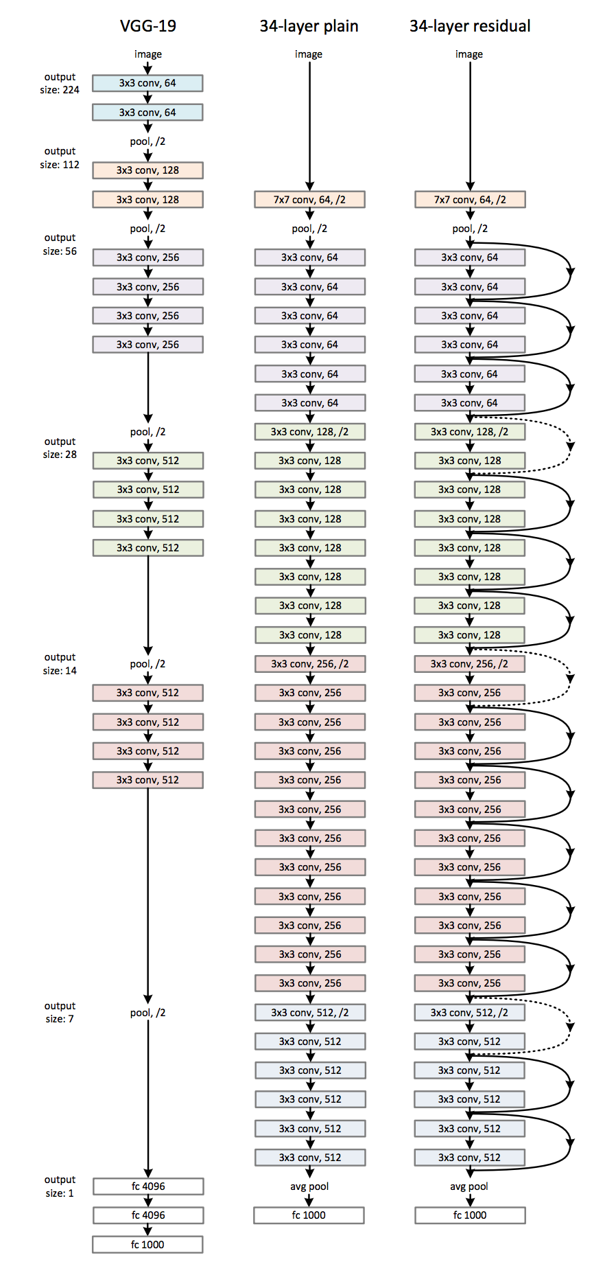
Their 200-layer ResNet won the 1st place in the ILSVRC classification last year. I highly recommend reading the original paper. I personally think that this idea might be a 2nd boom to field of computer vision since AlexNet from 2012.

The first ResNet-based network I experimented with was somewhat similar to the paper’s CIFAR10 network with n=3, resulting in 19 layers with 9 shortcut layers. I chose the CIFAR10 network structure first because a) I needed to verify if my implementation was correct at all, b) the images the classifier would be fed in were aligned already so it should not require a highly nonlinear and huge network.

I’d like to emphasize here my ResNet implementation was my own interpretation and might not be correct at all and might not be consistent with the original authors’ implementation.

I then tried to replicate the 50-layer ResNet with bottlenecking (see Table 1 of the paper). This configuration overfitted very quickly possibly due to the “width” of the network. So I followed the advice in section 4.2 and regularized the network by reducing the number of filters, and the network overfitted much later in the training process. I did not use bottlenecking after this point the filter sizes were not big.

Later I turned dropout back on and found that it helped prevent overfitting significantly. In fact I found that dropout higher than 0.5 (e.g. 0.8) improves the validation score even more.

Near the end of the competition, I also successfully trained a very deep and very thin ResNet with 67 layers. Below is its model definition:

l = nn.layers.InputLayer(
    name='in', shape=(None, 3, image_size, image_size)
)
# 256x256

l = conv2dbn(
    l, name='l1c1', num_filters=32, filter_size=(7, 7), stride=2,
    **conv_kwargs
)
# 128x128

l = nn.layers.dnn.MaxPool2DDNNLayer(l, name='l1p', pool_size=(3, 3), stride=2)
# 64x64

for i in range(3):
    l = residual_block(
        l, name='2c%s' % i,
        num_filters=48, filter_size=(3, 3),
        num_layers=2, **conv_kwargs
    )
# 64x64

for i in range(4):
    actual_stride = 2 if i == 0 else 1
    l = residual_block(
        l, name='3c%s' % i,
        num_filters=64, filter_size=(3, 3), stride=actual_stride,
        num_layers=2, **conv_kwargs
    )
# 32x32

for i in range(23):
    actual_stride = 2 if i == 0 else 1
    l = residual_block(
        l, name='4c%s' % i,
        num_filters=80, filter_size=(3, 3), stride=actual_stride,
        num_layers=2, **conv_kwargs
    )
# 16x16

for i in range(3):
    actual_stride = 2 if i == 0 else 1
    l = residual_block(
        l, name='5c%s' % i,
        num_filters=128, filter_size=(3, 3), stride=actual_stride,
        num_layers=2, **conv_kwargs
    )
# 8x8

l = nn.layers.dnn.Pool2DDNNLayer(l, name='gp', pool_size=8, mode='average_inc_pad')
l = nn.layers.DropoutLayer(l, name='gpdrop', p=0.8)

l = nn.layers.DenseLayer(l, name='out', num_units=n_classes, nonlinearity=nn.nonlinearities.softmax)

Interestingly, comparing with SGD, the ADAM optimizer led to more stable validation loss. Also, comparing with the 19-layer OxfordNet, the 67-layer ResNet was faster per epoch but slower to reach similar validation loss. However I have not confirmed if it was simply because of unoptimized learning rates.

At the end, I still had a lot of questions about how to best apply residual training to neural network. For example, if residual learning is so effective, would learning the residual of the residual error be even more effective (shortcut of shortcut layer)? Why does the optimizer has difficulty learning the original mapping in the first place? Can we combine ResNet with Highway Network? If the degradation problem is largely overcome, are the existing regularization techniques (maxout, dropout, l2 etc.) still applicable?

5.2 Inception v3

Following the success I had with ResNet, I decided to also replicate the other top performer of the ILSVRC challenge – Inception v3.

I tried to train the Inception net with no modification to the configuration at all except to add a dropout before the last layer, and no surprises it overfitted very quickly. Then I removed some of the “modules” to reduce its size, but I found the network still overfitted significantly. Note that I did not attempt to reduce the filter size because I was not sure how the number of filters were derived in the first place.

I did not ended up using the Inception network in the final ensemble.

5.3 Scaling training horizontally and Idea Validation

Because of my late start, the lengthy neural network training process became a huge problem. Most models used for submission took at least 36 hours to fully converge. So I bought an old GTX670 to optimize the hyperparameter for the aligner, while I used my main GTX980Ti for the classifier.

I found that having additional graphics card was much more helpful than having a faster graphics card. So one week before the deadline, I hacked together a system that allowed me to easily train a model on AWS EC2 GPU instances (g2.xlarge) as if I was training it locally, by running this command.

eval “$(docker-machine env aws0x)”
docker run -ti \
    -d \
    --device /dev/nvidia0:/dev/nvidia0 \
    --device /dev/nvidiactl:/dev/nvidiactl \
    --device /dev/nvidia-uvm:/dev/nvidia-uvm \
    -v /mnt/kaggle-right-whale/cache:/kaggle-right-whale/cache \
    -v /mnt/kaggle-right-whale/models:/kaggle-right-whale/models \
    felixlaumon/kaggle-right-whale \
    ./scripts/train_model.py --model … --data --use_cropped --continue_training

The model definitions were built as part of the container image. The whale images were uploaded to S3 from my local machine when necessary and were mounted inside the container. The trained models were then synced back to the S3 every minute and then to my local machine.

There are still quite a lot of quirks to be worked out. But this system allowed me to optimize the neural network hyperparameters that would have taken one month locally. Most importantly, I felt more “free” to try out more far-fetched ideas without slowing down ongoing model training. At peak, 6 models were training at the same time. Without this system, I would not be able to make an ensemble used in the final submission in time.

You can find the source code of this system on Github (felixlaumon/docker-deeplearning)

6. Final Submission

The final submission was an ensemble of 6 models:

• 3 x 19-layer OxfordNet
• 1 x 31-layer ResNet
• 1 x 37-layer ResNet
• 1 x 67-layer ResNet

The outputs of the global averaging layer were extracted and a simple logistic regression classifier were trained on the concatenated features.

I tried to perform PCA to reduce the dimensionality of the extracted features but found no improvements to the validation score.

A funny sidenote – 24 hours before the final deadline, I discovered that the logistic regression classifier was overfitting horrendously because the model accuracy on the training set was 100% and logloss was 0. I was in full-on panic mode for the next 12 hours because I thought something must have gone horribly wrong. Later I realized that the features were extracted with all non-deterministic layers turned off (esp. the p=0.8 dropout layer), and that was why it did not match the training loss (which was measured with dropout turned on). I wondered if monitoring training loss without dropout turned off would be a useful way to see if the network was overfittng or not.

7. Unimplemented Approaches

Here are some more ideas that should yield significant score improvement. But I was not able to finish implementing them fully before the deadline.

If you attempted any of these approaches or have any suggestion, please leave a comment below as I am very interested in how these ideas could have been panned out.

7.1. Reposing the Problem to Generate More Training Data

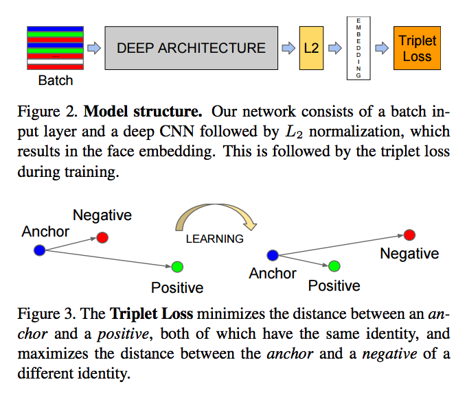
As mentioned before, one of the main challenges was the uneven distribution of number of images per whale, and the limited number of images in general. To avoid this problem, we can first repose the task as to identify if a pair of images belong to the same whale or not. Then we can train a classifier to learn an embedding which maps the whale images into compact feature vectors. The objective of the classifier was to maximize the euclidean distance of the feature vectors that contains the different whales, and minimize the distance with same whales. This idea was largely based on FaceNet.

I briefly experimented with this approach with a Siamese network with the contrastive loss function, but it did not converge. The network was trained with pairs of images which half of them were the same whale and the other half were different. I suspected that the online triplet image mining method used by FaceNet was actually essential to successful convergence.

7.2. Joint Training of Whale Aligner and Classifier

I briefly tried to apply Spatial Transformer Network (ST-CNN) to merge the aligner and the classifier. I expected good result because the localization and classification would be trained end-to-end.

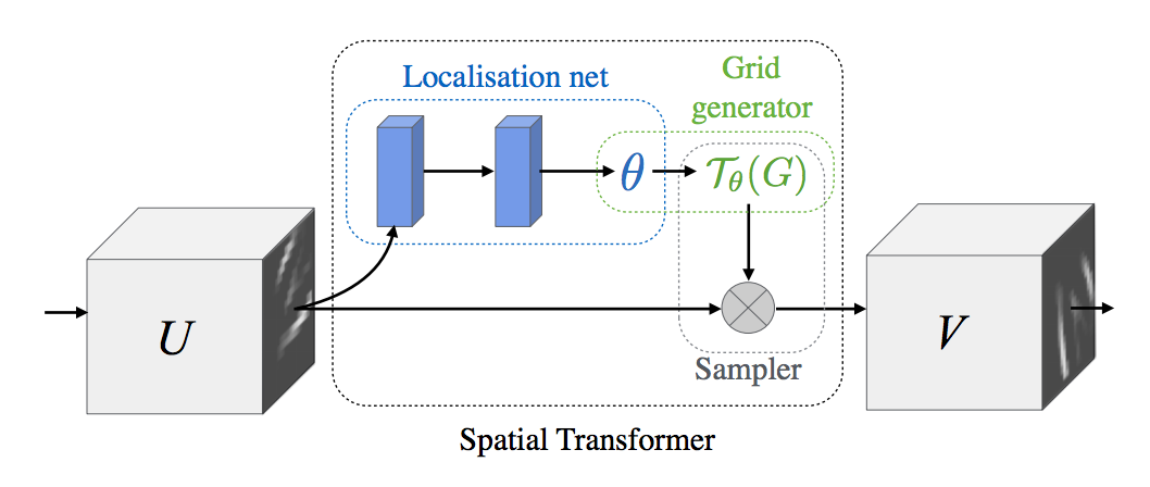
I was particularly confident that ST-CNN would work well because it achieved start-of-the-art performance on the CUB-200-2011 bird classification dataset using multiple localizers. (Arguably bird classification is much less fine grained than whale recognition. e.g. colors of birds of different species vary a lot, but not for whales). The diagram below shows samples from the bird dataset, and where the localizers focussed onto.

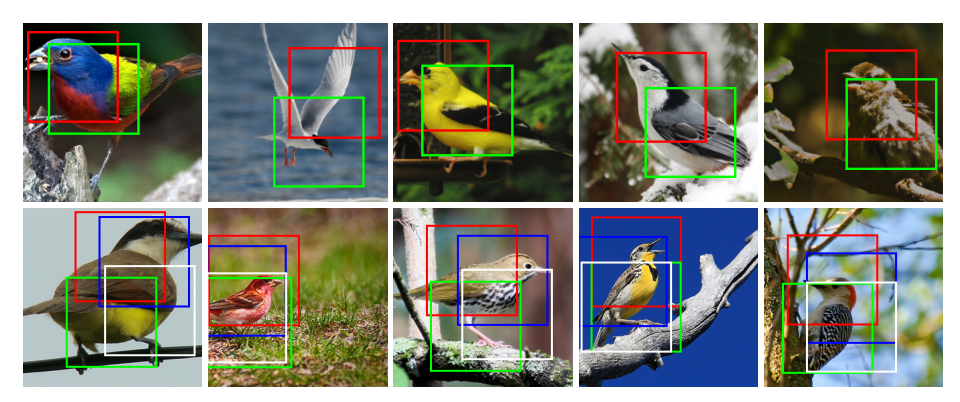
The first ST-CNN model was trained with 512x512 images and unfortunately, it was making random transformation, e.g. zooming in waves instead of the whale head. While I could not eliminate if this was due to a bug in my implementation, this echoed the result of the saliency map from section 4.1. I believed my explanation before applied here as well – the whale labels alone did not provide a strong enough training signal.

So in my next attempt, I tried to supervise the localization net by adding a crude error term to the objective function – the MSE of the predicted affine transformation matrix and the actual matrix generated by the bonnet and blowhead annotation. Unfortunately, I was not able to compile this network with Theano.

So it remained an open question for me – Can localization network of ST-CNN be trained in a supervised manner? Will semi-supervised training further improve the performance of ST-CNN?

One approach I did not try was 1) pre-train localization network to learn the affine transformation that would align the image to the whale’s blowhead and bonnet, 2) follow normal procedure to train the whole ST-CNN. Perhaps in the 2nd stage, the learning rate must be reduced to prevent the localizer from drifting away from whale head. It might also be a good idea to pretrain the classification part as well to prevent the need of manually adjusting the learning rate altogether. This is something I would have attempted if I had more time.

I am particularly interested in understanding how ST-CNN should be applied to this dataset. Please contact me if you have any suggestions.

7.3. Transfer Learning

Transfer learning offers an alternative way to reduce training time, other than to simply spawning more GPU instances.

For training networks with same architecture and configuration, I could have simply load the weights learned from a previous network. However, for networks with different number of layers or filters, loading weights from a similar network doesn’t seem to work very well. In fact, most of the time it was worse than without using the learned weights! Transferring learned features to a slightly different network was a much more common use case because my goal was to optimize the number of filters and number of layers

I investigated briefly with Net2Net but wasn’t able to implement its algorithm.

7.4 Pre-training

Pre-training the classifier with test images might have helped because the testing set had more images than the training set. Combining with section 7.1, we could even apply the learned embedding to the test set to generate labels. I expected this might lead to better result than pseudo-labelling.

8. Conclusion

I had a lot of fun working on this challenge, and I learned a lot when trying to find new and interesting ideas from academic research. The last 3 weeks were very exhausting for me, because there were so much to do and I was working alone! Next time I would definitely team up.

I’d like to congratulate other winners and other top performing teams and contestants. I am still amazed by the progress we made in the leaderboard in the last 3 weeks!

I strongly encourage you to check out the competition forum as there have been many alternative approaches shared throughout the competition. In particular, I am surprised by the number of non-deep-learning approach with localizing the whale! e.g. unsupervised physics based whale detector, detector based on principle components of color channel, histogram similarity, mask based regression

Finally, I’d like to thank Kaggle for hosting this compeitition, and MathWorks for sponsoring and providing a free copy of MATLAB for all participants. Of course this was not possible without NOAA releasing this rare dataset and the huge effort from Christin Khan and Leah Crowe for hand labelling the images! I hope we will see more datasets from NOAA? ;)

If you have any questions or feedback, please leave a comment below.

Follow me on Twitter @phelixlau.

Update 1: See further discussions about this blog post at r/machinelearning

Update 2: The source code is now available at https://github.com/felixlaumon/kaggle-right-whale